| Design and Data Processing Principles of a GNSS-R Receiver with a DDMI Jyh-Ching Juang Distinguished Professor, Department of Electrical Engineering, NCKU |
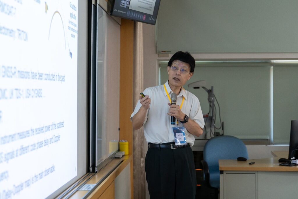
Distinguished Professor Jih-Ching Chuang from the Department of Electrical Engineering, National Cheng Kung University, delivered a lecture titled “Design and Data Processing Principles of a GNSS-R Receiver with a DDMI,” providing an in-depth analysis of the GNSS-R receiver carried by TASA’s (Taiwan Space Agency) recently launched Triton satellite and its data processing techniques. The lecture highlighted Triton’s potential in ocean observation, weather forecasting, and other fields, while emphasizing Taiwan’s significant achievements in space technology development.
Triton Satellite: The Wind Hunter of the Ocean
Professor Chuang introduced Triton as TASA’s newest satellite, which has been in orbit for almost two years. The satellite’s core mission is to be a “wind hunter,” aiming to deduce critical data such as ocean wind speed, sea surface roughness, and soil moisture by collecting information from GNSS (Global Navigation Satellite System) signals reflected off the Earth’s surface. Triton operates in a sun-synchronous Low Earth Orbit (LEO) at approximately 600 kilometers, and its GNSS-R receiver can pick up reflected signals from GPS, BeiDou, GLONASS, and other GNSS satellites.
GNSS-R Technology: Advantages of Passive Observation
The principle of GNSS-R technology is to utilize GNSS satellites as sources of “signals of opportunity,” where the on-board instrument only needs to receive these reflected signals without carrying a transmitter. This “passive” reception method allows for the miniaturization of satellite payloads, reducing the need for large satellites and high power, aligning with the recent trend of “new space” development. Professor Chuang noted that reflected signals, after scattering from the Earth’s surface (such as the ocean), experience variations in delay and Doppler frequency due to surface roughness, wind speed, and other factors. These variations, once captured by the receiver, can generate two-dimensional “Delay Doppler Maps” (DDM), which are then used to infer surface information. This technology has been explored in missions such as the UK’s DMC and TDS-1, and NASA’s CYGNSS in the United States, used to predict typhoons and cyclones.
Instrument Design and Challenges
The GNSS-R receiver on the Triton satellite is a critical instrument, with its design and development spanning nearly a decade, from its initiation in 2014 to its successful launch in 2023. The instrument is equipped with a nadir-pointing antenna array (evolving from four elements to eight elements) to capture weak scattered signals. Key design challenges include: extremely weak signals, dynamic changes in Doppler effects, and high demands for real-time processing capabilities. To address this, the team developed fast computation algorithms and utilized Fast Fourier Transform (FFT) techniques to generate DDMs. Additionally, the receiver must be precisely synchronized and capable of calculating the signal’s “specular reflection point” to ensure accurate DDM localization.
Triton’s GNSS-R receiver is primarily designed for GPS L1 signals, but its open-format characteristic allows for future expansion to other GNSS systems (such as Galileo, QZSS, BeiDou, GLONASS) and multiple frequency bands (L2, L5). The receiver can generate four DDMs per second, each with 128 code phases and 64 Doppler shifts, a performance that surpasses some existing missions (e.g., NASA’s CYGNSS satellite).
Initial Observation Results and Data Applications
After its launch on October 9, 2023, the Triton satellite successfully powered on and began operation within just three days, demonstrating the rapid response capabilities of new space missions. Current observations focus on ocean wind fields in the Pacific, Indian, and Atlantic Oceans.
Initial operational results indicate:
• DDM Validation: The received DDMs exhibit expected shapes and energy distributions, and can differentiate between characteristics of ocean and land reflected signals.
• Data Quality: Six to eight DDMs can be received per second, and their accuracy has been verified through metadata.
• QZSS Signal Reception: Triton is capable of successfully receiving signals from Japan’s Quasi-Zenith Satellite System (QZSS), a unique capability not present in other similar missions (such as CYGNSS).
• Data Release: All requirements have been met, and the relevant data has been made public, allowing interested researchers to register and download it.
Data Processing and Advanced Applications
Professor Juang further shared research achievements on advanced applications of GNSS-R data. The research team utilized deep learning techniques, such as CNN and CNN-LSTM, for ocean wind speed retrieval, currently achieving an accuracy of approximately 1.7 meters/second. Furthermore, they are exploring the potential of Triton data for typhoon monitoring, observing changes in observations as wind speeds vary from low to high.
A particularly notable innovation is the development of a DDM classification network. As DDM data can sometimes be affected by interference signals (interference DDM) originating from the ground, especially in specific border regions of certain countries (e.g., the Russian-Ukrainian border), these interference signals can impact data usability. The research team developed a classification network that can effectively identify and categorize “horseshoe-shaped” ocean reflections, specular reflections (specular class), and interference signals. This technology helps to remove interference during the data processing phase or filter out specific types of DDMs for analysis, thereby improving data quality and application scope.
Conclusion
The successful development and operation of the Triton satellite’s GNSS-R payload is the culmination of a collaborative effort between TASA, National Cheng Kung University (NCKU), and National Central University (NCU), with special thanks to Professor Yang and Professor Chen, among other team members. Professor Juang’s lecture demonstrated Taiwan’s strong capabilities in autonomous space instrument development, data processing, and advanced applications, injecting new momentum into global ocean and meteorological scientific research.
| High-Frequency Ocean Doppler Radar Design and Data Analysis Hwa Chien Distinguished Professor, Graduate Institute of Hydrological & Oceanic Sciences, NCU |
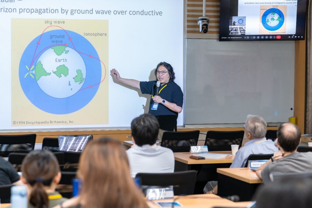
HF Radar: The Unique “Over-the-Horizon” Eye for Ocean Observation
Professor Hwa Chien’s lecture provides an in-depth look into the fundamental principles, design, and data analysis of High-Frequency Ocean Doppler Radar (HF Radar), emphasizing its unique value in oceanographic applications. This radar operates in the frequency range of 1 MHz to 30 MHz, which is significantly lower compared to the microwave L-band (gigahertz) used by GNSS signals. Its most distinctive characteristic is its utilization of the “ground mode” propagation, allowing electromagnetic waves to diffract along the interface between the air and “saltwater ocean”. This technology grants HF radar “over-the-horizon” observation capabilities, enabling it to “see over the horizon”. Professor Chien highlighted that HF radar is currently the only technology capable of 24/7 continuous monitoring of sea areas for 20 years without interruption, a feat unmatched by other technologies.
Capturing Faint Signals: Bragg Scattering and Coherent Integration
The core principle behind HF radar operation is receiving “Bragg scattered” signals from ocean waves. However, these backscattered signals are extremely weak, approximately six orders of magnitude (one million times) weaker than specular reflection. To overcome this challenge, HF radar employs “coherent integration” techniques, accumulating signals over extended periods (e.g., 30 minutes) to significantly improve the signal-to-noise ratio, thereby effectively detecting these faint signals. Bragg resonance requires the wavelength of ocean surface waves to be approximately half the radio wavelength. As the ocean surface is composed of an infinite number of random wave components, there will always be at least one component that satisfies the resonance condition, ensuring stable signal reception.
Doppler Spectrum Decoding Ocean Dynamics
Key ocean parameters can be extracted from the received Doppler spectrum of HF radar. When radar waves resonate with ocean “gravity waves” via Bragg scattering, a “first-order peak” is produced, whose Doppler shift is related to the wave speed. If ocean currents are present, they further modulate the wave’s speed, causing changes in the Doppler shift, which allows for the inference of “radial current velocity”. Additionally, the “second-order peak” in the spectrum can be used to estimate the “ocean wave spectrum”, while the difference between the first and second-order peaks can be utilized to measure wind direction and wave direction.
Self-Assembled Radar Systems and Efficient Data Processing
Professor Chien’s team primarily develops “Continuous Wave” (CW) radar systems. Such a system requires only 30 watts of low power to achieve a monitoring range of 200 kilometers. The radar employs a simple, low-cost “homodyne radar” structure. To measure range, the radar transmits “linear chirp” signals (similar to GNSS C/A code) and calculates distance by comparing the “frequency difference” between transmitted and received signals, rather than traditional pulse time-of-flight. The data processing steps involve: first “demodulating” the received signal to obtain the “beat frequency”, followed by a second Fast Fourier Transform (FFT) to generate the Doppler spectrum. To ensure high precision, radar systems have strict requirements for clock synchronization, often using GPSDO’s one-pulse-per-second (PPS) signal or atomic clocks to synchronize transmitters and receivers. Professor Chien’s team has deployed approximately 20 self-assembled HF radar stations along Taiwan’s coast.
Similarities and Differences with the Triton Satellite Mission
Professor Chien also drew comparisons between HF radar and TASA’s Triton satellite mission. Both operate in a “bi-static mode,” meaning the transmitter and receiver are located at different positions. However, the main difference lies in Triton satellite’s GNSS Reflectometry being a vertical observation from orbit, whereas HF radar performs horizontal observations from the coast. Despite their differing technical principles, HF radar and GNSSR share similarities in data processing steps, such as demodulation, matched filtering, and coherent integration, with the ultimate goal of extracting key ocean parameters like wind, waves, and currents from surface observations.
| Introduction of Triton v2.0 ocean surface wind speed product Wen-Hao Yeh Associate Researcher, TASA |
Introduction of Triton v2.0 Ocean Surface Wind Speed Product: Enhanced Accuracy and Future Prospects
Dr. Wen-Hao Yeh, Associate Researcher at the Taiwan Space Agency (TASA), provided a detailed presentation on the development of the Triton version 2.0 (v2.0) ocean surface wind speed product, its key improvements, and TASA’s future satellite mission plans. This update aims to provide more accurate and reliable global ocean surface wind speed data, holding significant implications for meteorological forecasting and oceanographic research.
Overview of Triton Satellite Mission and Data Processing
Dr. Yeh began by briefly introducing the Triton satellite mission and its onboard Global Navigation Satellite System Reflectometry (GNSSR) payload. The Triton satellite features two antennas: a high-gain antenna directed towards the Earth’s surface to receive reflected GPS signals from the ocean, and another pointing zenith to receive direct GPS signals for satellite positioning. The core measurement of GNSSR is the Delay Doppler Map (DDM), which records the strength of reflected signals across different delays and Doppler shifts. As the ocean surface is not a perfect reflector, the DDM captures not only signals from the specular point but also scattered signals from surrounding areas.
The data retrieval process consists of four main segments: data format transfer, DDM calibration, calculation of Effective Scattering Area (ESA) and Normalized Bistatic Radar Cross-Sections (NBRCS), and finally, ocean surface wind speed retrieval.
Key Improvements in Version 2 Ocean Surface Wind Speed Product
1. Refined DDM Calibration Dr. Yeh emphasized the necessity of DDM calibration due to the influence of the receiver and antenna on raw DDM data. Version 2 introduces improved methods for calculating signal power (G-value), particularly in the absence of reference instruments like black body radiators. This is achieved through statistical analysis. To address abnormally high noise floors, the team designed nine cases to remove “expanded data.” Comparing these results with European Centre for Medium-Range Weather Forecasts (ECMWF) wind speed data, Case 4 was found to yield the best calibration, significantly enhancing data quality.
2. Specular Point Determination and NBRCS Calculation Regarding specular point determination, Version 1 employed a sliding process that was less effective with weak signals. Version 2 integrates the WGS84 geodetic system and DT10 mean sea level data to adjust the Earth’s surface height, allowing for more precise determination of the specular point’s delay and Doppler shift. The sliding process is still used for clear signals as a complementary method.
NBRCS calculation is fundamental for wind speed retrieval. Triton products provide NBRCS values for three different grid sizes: 1×1, 3×5, and 13×21 pixels. Dr. Yeh explained that using larger grids can reduce the influence of signal ambiguities in the DDM but at the cost of spatial resolution (approximately 25 kilometers).
GMF Development and Wind Speed Retrieval Results
1. Development of Geophysical Model Function (GMF) The GMF is an empirical model that converts NBRCS into ocean surface wind speed. Version 2’s GMF development not only classifies data based on signal inclination angles but also further differentiates by the PN code and number of GPS satellites. A crucial improvement is the incorporation of corrections based on the satellite’s relative velocity directions, which significantly enhanced data convergence compared to uncorrected data.
2. Improved Wind Speed Retrieval Accuracy In terms of wind speed retrieval accuracy, Version 2 products show a Root Mean Square Error (RMSE) of approximately 2.25 m/s, a notable improvement over Version 1’s 2.7 m/s.
3. High Wind Speed Mode and Typhoon Data To address high wind speed conditions, Version 2 specifically developed a high wind speed mode GMF, trained using simulated typhoon data. Dr. Yeh noted that while there remains a gap between the mean NBRCS curves for high and low wind speed modes, using smaller grid numbers for NBRCS calculation can help reduce this discrepancy. For instance, during Typhoon Podul, Triton detected wind speeds exceeding 10 m/s in the typhoon eye region, and up to 30 m/s in the high wind speed mode.
Future Outlook: TASA Satellite Mission Plans
Dr. Yeh also outlined TASA’s future satellite mission plans. In addition to the current Triton and the retired FORMOSAT-3 and operational FORMOSAT-7, TASA has decided to incorporate GNSSRO receivers as secondary payloads on FORMOSAT-9, 9A, 9B, and FORMOSAT-8E, 8F satellites. These new payloads will enable simultaneous Radio Occultation (RO) and reflectometry observations, expanding the application scope of GNSSR to include atmospheric and ionospheric profiling, soil moisture, water body mapping, and sea ice distribution studies. Although GNSSRO receivers will be turned off during Synthetic Aperture Radar (SAR) observations and downlink transmissions due to satellite attitude changes, these future missions are projected to significantly increase daily observations, with approximately 300,000 reflection observations and 800-900 multi-GNSS RO profiles per day.
Data Access and Future Development
Dr. Yeh concluded by announcing that Triton Version 1 products were released at the end of May 2024, and Version 2 products were released on August 22, 2024. Interested users can freely register and download Triton data, as well as FORMOSAT-7 and FORMOSAT-3 data, from the websites of the Taiwan Analysis Center for Cosmic (TACC) or the Central Weather Administration (CWA). In the future, TASA aims to continuously provide RO and reflectometry data through new satellite constellations, further advancing Earth science research.
| Pulsar Scintillation Arcs: Direction and Speed of Interstellar Waves Daniel Thomas Baker Postdoc Fellow, Institute of Astronomy and Astrophysics, Academia Sinica |
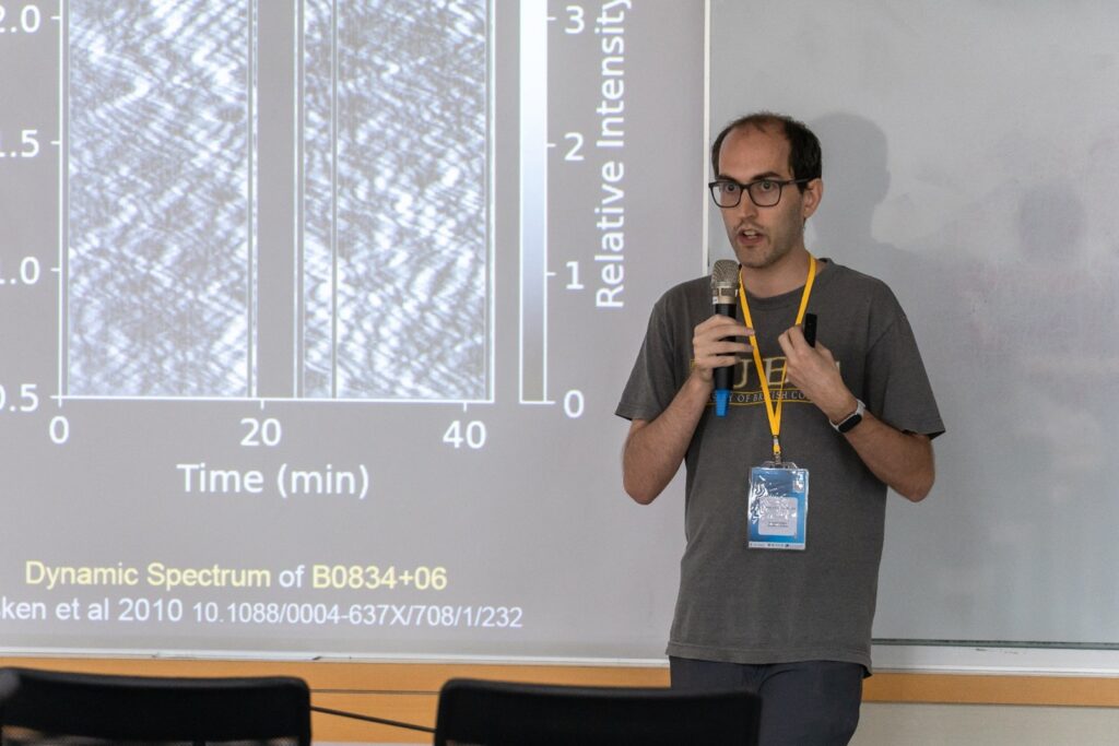
Dr. Baker’s research focuses on leveraging pulsar scintillation to characterize the interstellar medium. While his approach might seem “very unrelated” to current problems, he has proposed a novel technique to extract more information from Delay-Doppler Map (DDM) products. His work primarily involves pulsars and their scintillation, aiming to understand the fine structures within the ISM by analyzing how radio signals refract as they propagate through interstellar space.
Pulsar Scintillation: Cosmic “Ocean Reflections”
Pulsars emit highly regular pulsed signals. As these signals travel to Earth, they propagate through the ISM, where variations in electron density cause the signals to refract. This refraction can lead to multiple paths for the signal to reach Earth, creating an interference pattern. Dr. Baker draws an analogy, stating that just as one might study reflections off the ocean surface to understand ocean dynamics, his team examines refraction through the ISM to
comprehend its internal structures. Their primary interest lies in characterizing the impulse response, or equivalently, the frequency response, of the ISM—what they term the “wave field”.
However, a significant challenge arises because individual pulsar pulses behave very differently, exhibiting random phases, varying shapes, and fluctuating intensities. This precludes simply averaging multiple pulses to analyze the complex response, as random phases would cancel each other out.
Dynamic and Conjugate Spectrums: Decoding Cosmic Interference Patterns
To overcome this, the research team examines the “dynamic spectrum,” which represents the averaged pulse intensity of the pulsar as a function of time and frequency. Essentially, it’s the amplitude squared of the wave field. This spectrum displays a characteristic “crisscross pattern”.
They then perform a 2D Fourier transform on the dynamic spectrum to obtain the “conjugate spectrum,” which is a “cousin” to the Delay-Doppler Map. The conjugate spectrum shows the power as a function of time delay and Doppler shift. A prominent feature within it is a clear parabolic structure, along with secondary parabolas referred to as “inverted arclets”. These inverted arclets are copies of the main parabola, with their apices situated along it.
The Mystery of the Arcs: Clues to Interstellar Medium Structure
These arcs pose crucial questions: What can be learned from them? Can they be used to recover the underlying complex phases of the ISM’s response function, a problem known as “phase retrieval”?
Dr. Baker explains that the conjugate spectrum is the self-convolution of the 2D Fourier transform of the wave field (termed the conjugate wavefield). The simplest explanatory model involves a single scattering screen at a specific distance, where all scattering points lie in a single direction on the sky. In this scenario, Doppler shifts are proportional to the angular offset, and time delays are proportional to the square of the angular offset. This leads to a quadratic relationship between time delays (TOA) and Doppler shift, characterized by a “curvature” parameter (η), which is inversely proportional to the square of the projected velocity.
Rich Information from Curvature Measurements
Measuring variations in this curvature can reveal a wealth of information:
• Annual variations: Due to Earth’s orbital velocity changes around the sun, which affect the projected velocity, causing annual variations in the measured curvature.
• Binary pulsar oscillations: If the pulsar is in a binary system, its own motion induces secondary oscillations.
• Screen orientation and velocity: By projecting Earth’s known orbit and the pulsar’s direction onto the sky, the spatial orientation and velocity of the scattering screen, as well as the center of mass motion of a binary system, can be inferred.
• Precise binary orbits: Information about the scattering screen also helps to fill in additional details about the binary’s orbit.
Furthermore, Very Long Baseline Interferometry (VLBI) can be used to pinpoint the sky location from which individual points in the conjugate spectrum originate, revealing a straight collection of scattering images on the sky.
Solving the Phase Retrieval Problem: Unveiling the Wave Field
Dr. Baker dedicates much of his time to solving the “phase retrieval problem”. The conjugate spectrum is the self-convolution of the underlying conjugate wavefield. Each point in the spectrum contains information about the interference between a pair of images on the sky. If there are ‘n’ images, there are n^2 pairs, but only ‘n’ complex magnifications to solve for.
They map the spectra into a different space called “theta-theta space”. This mapping allows them to simplify the deconvolution problem into a more tractable eigenvalue decomposition problem. This mapping is highly sensitive to the chosen curvature: a correct curvature yields clear vertical and horizontal lines, while an incorrect one results in skewed or collapsed structures. By analyzing the power in the dominant vertical and horizontal structures, they can achieve order-of-magnitude improvements in curvature measurements.
Enhanced Measurement Techniques and Applications
Once the wave field is successfully recovered, additional physical constraints are applied. For example, all image time delays (tow) must be greater than zero (as signals cannot arrive faster than the direct line of sight). These constraints help to relax earlier assumptions of purely one-dimensional scattering, enabling the detection of more complex, non-one-dimensional scattering structures, such as “wobbles” or additional “isolated” clumps of images observed in the sky map.
ISM’s “X-ray Vision”: Probing Fine Structures
This research has also yielded fascinating insights and applications:
• Second Scattering Structure: They identified a distinct “millisecond feature,” an isolated group of images, which may represent an additional blob of material in the ISM acting as a secondary lens. The light might scatter off this secondary lens first, and then off the main screen.
• Probing Electron Column Density: Because different scattering paths traverse slightly different regions of the ISM, each image path probes a unique electron column density.
• Dispersion Measure Variation: An increased electron count causes lower frequencies to arrive later. By tracking individual images and observing how their time delay evolves with frequency, they can identify regions of reduced or enhanced electron column density on either side of the line of images. This provides an invaluable tool for probing the fine structures of the ISM.
Dr. Baker also briefly mentioned a toy model that compares these phenomena to reflections from a single wave on the ocean surface. He noted that by analyzing how curvature evolves over time and sky position, it might be possible to distinguish between multiple potential solutions for the scattering screen parameters.
| Improving the Retrieval Capability of the Triton Satellite under High Wind Speed Conditions Using a Neural Network Model Shih-Chiao Tsai Director, Department of Environmental Information and Engineering, NDU |

Overcoming Limitations in High Wind Speed Satellite Retrieval
Director Shih-Chiao Tsai from the Department of Environmental Information and Engineering, National Defense University, recently unveiled groundbreaking research on improving the retrieval capability of the Triton satellite under high wind speed conditions using a neural network model. This pivotal study aims to resolve a critical issue in traditional Triton Geophysical Model Function (GMF), where the sensitivity of the Differenced Delay-Doppler Map Average (DDMA) diminishes at high wind speeds, consequently limiting the accuracy of wind speed retrieval.
Background: The Challenges of Conventional Methods
Triton satellite technology is highly regarded for its robust availability and reduced susceptibility to surface disturbances such as heavy rain. Its operational principle involves using the DDMA near the specular point to establish the GMF, which then infers wind speed. However, a significant limitation arises: as wind speeds intensify, the DDMA’s sensitivity declines, leading to a considerable reduction in the accuracy of wind speed retrieval under high wind conditions. To surmount this challenge, the research team pivoted to employing neural networks for training Triton satellite feature data.
Innovative Approach: AI Models and Multi-Source Data Integration
The core of this research involved leveraging two advanced artificial intelligence models: the Feed Forward Neural Network (FNN) model and the Long Short-Term Memory (LSTM) model. The team meticulously collected data from various sources, including Triton satellite data (DDM power, ocean surface wind speed, Mean Square Slope (MSS), and Significant Wave Height, with data coverage from October 2023). Additionally, ERA5 reanalysis data from the European Centre for Medium-Range Weather Forecasts (ECMWF), providing wind speed, significant wave height, and MSS, was integrated. To further explore future application potential, the team also developed a self-built WRF (Weather Research and Forecasting) model simulation, converting simulated wind speeds to MSS for AI model training.
Regarding data preprocessing, the team executed rigorous steps, including antenna gain correction, Doppler axis correction, quality control, and spatial and temporal interpolation. Furthermore, feature engineering was applied, scaling data ranges to 0-1 and transforming periodic features like time and azimuth into cyclic sine forms. Notably, inspired by NASA’s CYGNSS satellite’s GMF which utilizes both Leading Edge Slope and DDMA, the research team also devised a method to derive the leading edge slope from Triton data.
Key Finding: The Decisive Role of Mean Square Slope (MSS)
The research findings unequivocally highlight that Mean Square Slope (MSS) is a critical feature for enhancing model prediction accuracy. For both FNN and LSTM models, the inclusion of MSS in the training dataset led to a significant improvement in performance, even outperforming WRF model simulation results. MSS effectively describes the roughness of the sea surface and exhibits a positive correlation with wind speed. The study further revealed that leading edge slope, NBRCS, and DDMA have a negative correlation with wind speed, whereas MSS shows a positive correlation. This strongly underscores the critical role of external physical covariates in accurate wind speed retrieval.
Model Performance and Future Outlook
In terms of model performance comparison, the FNN model proved to be more suitable for processing Triton satellite data, primarily because Triton data is not a typical time-series dataset. In contrast, while the LSTM model is designed for handling time-series data, its performance in this study was not as robust as FNN. The research data demonstrated that with the inclusion of external parameters like MSS, the FNN model’s Root Mean Square Error (RMSE) significantly decreased from approximately 2.8 for the original GMF to 1.2-1.6, marking a substantial improvement in prediction accuracy under high wind conditions.
Director Tsai concluded that despite the current underrepresentation of high wind speed records in the training dataset, future efforts must focus on increasing the proportion of high wind speed samples to further optimize model performance. This research not only successfully enhanced the Triton satellite’s wind speed retrieval capability in high wind conditions but also provided invaluable experience and a foundation for future applications of satellite data in meteorological forecasting.
| Atmospheric Applications of GNSS Radio Occultation Data and Prospects for Polarimetric RO Observations Shu-Ya Chen Associate Researcher, Global Atmospheric Observation and Data Applications Research Center, NCU |

Dr. Shu-Ya Chen, Associate Researcher at the Global Atmospheric Observation and Data Applications Research Center, NCU, delivered a lecture titled “Atmospheric Applications of GNSS Radio Occultation Data and Prospects for Polarimetric RO Observations.” The talk focused on the practical applications of Radio Occultation (RO) data, rather than its processing, specifically exploring its potential in tropical cyclone forecasting and the use of Polarimetric RO (PRO) observations for evaluating microphysics parameterizations in numerical models.
GNSS Radio Occultation: Principles and Broad Applications
The lecture began with a brief introduction to the GNSS Radio Occultation (RO) technique. When signals from GNSS satellites pass through the Earth’s atmosphere, they bend and experience a phase delay due to air density. By deriving the bending angle and refractivity from these measurements, scientists can further obtain crucial atmospheric parameters such as temperature, pressure, and water vapor pressure.
RO data has a wide range of applications, including climate monitoring, detection of Planetary Boundary Layer (PBL) height, and daily weather forecasting in major operational weather centers globally. An assessment by the European Centre for Medium-Range Weather Forecasts (ECMWF) demonstrated that integrating RO data from FORMOSAT-7 and commercial Spire data into their operational system immediately showed significant positive contributions, effectively reducing forecast errors.
RO Data Assimilation Enhances Tropical Cyclone Forecasting
Experimental Design and Case Analysis
Dr. Chen presented a study conducted by her team to assess the impact of RO data assimilation on the prediction of tropical cyclogenesis. The study utilized 10 typhoon cases in the Northwest Pacific (2020-2022), employing the WRF numerical model with a hybrid 3DEnVar data assimilation system. Two experiments were conducted for each typhoon case: one without RO data assimilation and another with it. Within each three-day data assimilation cycle, approximately 2,000 to 3,000 RO soundings were used, with over 75% contributed by FORMOSAT-7.
The results indicated that without RO data assimilation, only 5 cases successfully predicted the cyclone formation. With RO data assimilation, the number of successful cases increased to 8. Furthermore, simulations with RO data assimilation showed significant improvements in the errors of genesis time and location, doubling the detection rate for genesis within a 24-hour time error.
Insights from Typhoon Chanthu
Focusing on Typhoon Chanthu in 2021 as a case study, the model failed to simulate genesis without RO data assimilation. However, with RO data assimilation, the model successfully simulated Typhoon Chanthu’s genesis, even 9 hours earlier than the best track, with minimal error. Further analysis revealed that RO data assimilation significantly increased moisture over the ocean, facilitating convergence and driving vertical motion, which ultimately contributed to tropical cyclone development.
The Critical Impact of RO Data Assimilation
Sensitivity tests highlighted that RO data within the precursor region near the genesis location is crucial; removing this data resulted in no genesis simulation for that case. Even when assimilating abundant satellite radiance data, the model still struggled to simulate Chanthu’s genesis without RO data. However, combining RO data assimilation with radiance data successfully captured the genesis. Moreover, in a 32-member ensemble forecast, all members successfully captured Typhoon Chanthu’s genesis with RO data assimilation, whereas zero cases were successful without it, further underscoring the importance of RO data assimilation.
Polarimetric Radio Occultation: Precipitation Detection and Microphysics Scheme Evaluation
Introduction to the Emerging PR Technique
The second part of the lecture focused on Polarimetric Radio Occultation (PRO), an emerging technique. The PRO observations using two linear polarized antennas (horizontal and vertical). When rays pass through oblate-shaped large raindrops, horizontal and vertical polarized signals experience different time delays and phase shifts. By measuring this “differential phase shift” (delta phi) along height, PRO technology has the potential to evaluate precipitation, including heavy rainfall events.
Uncertainties in Model Microphysics Schemes
Dr. Chen’s team further utilized PRO data as a diagnostic tool to evaluate microphysics parameterization schemes in numerical models. The study selected three typhoon cases from 2019 to 2021: Bualoi, Matmo, and Kompasu. Experiments used the WRF model, combining two different initial conditions and five microphysics schemes. The results showed that different initial conditions (e.g., ERA5 or NCEP FNL) and microphysics schemes led to significant differences in typhoon intensity and structure. For instance, track simulations for Typhoons Matmo and Kompasu exhibited clear northward/southward biases depending on the initial conditions. Initial track error verification suggested that the Goddard microphysics scheme performed slightly better in typhoon track simulations.
Diagnostic Capabilities of PRO Data
The differential phase shift (delta phi) from PRO observations is highly sensitive to precipitation intensity. Since delta phi is not a direct variable in models, a forward operator needed to be developed to convert the model variables into delta phi. To mitigate errors in typhoon simulations related to location, time, and cloud structure, the research team performed various pre-processing steps, including typhoon relocation and time interpolation.
Verification in the Case of Typhoon Bualoi
Using Typhoon Bualoi as an example, a comparison between model-simulated delta phi and PRO observations was conducted. The results indicated that the Goddard scheme and two-moment microphysics schemes (Thompson and Morrison) showed better agreement with PRO observations in terms of delta phi peak and structure, compared to other schemes. Ensemble forecast results further confirmed that the Goddard scheme, on average, captured the observed delta phi peak effectively.
Conclusion
Dr. Chen’s lecture concluded that GNSS Radio Occultation data plays a critical role in tropical cyclone forecasting, significantly improving the accuracy of genesis predictions. Simultaneously, the emerging Polarimetric Radio Occultation technique provides a powerful diagnostic tool for evaluating microphysics parameterization schemes in numerical models, which can help enhance the model’s ability to simulate precipitation events.
| Bias estmiation of Radio occultation data in the Deep Troposphere Shu-Chih Yang Director, Global Atmospheric Observation and Data Applications Research Center, NCU Gia-Huan Pham Global Atmospheric Observation and Data Applications Research Center, NCU |

Research Background and Data Application Challenges Radio Occultation (RO) is recognized as a crucial technique for probing the lower or deep troposphere (boundary layer) because it provides very high vertical resolution of temperature and moisture, thereby accurately depicting the thermodynamic structure of the planetary boundary layer (PBL). This makes RO data highly promising for Numerical Weather Prediction (NWP). However, current data assimilation systems reject over 70% of RO data below 2 kilometers due to strong biases in the deep troposphere, limiting their practical use. The research team initially succeeded in correcting refractivity profiles and has now advanced to the more challenging task of correcting bending angle biases. The COSMIC-2 (FS7) satellite is considered an improvement for retrieving more data in the deep troposphere and serves as an “anchor” observation for correcting other satellite observations, yet it still contains severe biases, especially in tropical and subtropical oceans.
Primary Sources of Bending Angle Bias in the Deep Troposphere Bending angle biases originate from multiple factors. Early RO signal processing assumed single-ray propagation, but multipath propagation is a real issue. Although open-loop processing and radio holographic methods introduced in 2011 have reduced multipath effects in the lower troposphere, these methods still rely on the key assumption of “spherical symmetry of refractivity”. In convective moist areas or layers with large refractivity gradients, this non-spherical symmetry introduces potential bias sources.
Specifically, moisture effects are a critical factor. Below 7.5 kilometers, moisture induces multipath propagation, causing the bending angle spectrum to broaden. Additionally, signal truncation introduces bias. If the signal is cut too early during processing (e.g., at 5 kilometers), it leads to an asymmetric spectrum, resulting in a negative bending angle bias in the low troposphere, particularly in regions with high near-surface moisture. Super refraction or ducting is another major source; when refractivity gradients are extremely large, signals can become trapped and reach the receiver without a tangent point, leading to singularity and large bending angle bias. This phenomenon generates a “D-signal” (delayed signal), but the D-signal is not always solely indicative of super refraction, as it can arise from other signal processing origins.
Innovative Approach: Machine Learning-Based Dynamic Bias Estimation Previous quality control methods (e.g., using single proxies like moisture gradients or local spectrum width) proved insufficient to characterize the complex nature of biases, as they vary with region and amplitude levels. Therefore, this study developed a dynamic bias estimation method using machine learning, incorporating multiple inputs to account for biases across different regions and levels.
The research utilized ATM/wet profiles (Level 2 data) and CONFYX profiles (1B data) from FS7 COSMIC-2, using ECMWF reanalysis data (ERA5) from December 2019 to May 2020 as “truth” for training. The Radio Occultation Processing Package (ROPP) served as a forward model to compute refractivity and bending angle from ERA5 data. Through spike detection techniques, bending angle biases were classified into four types: large negative geometrical bias (LNGB), large positive geometrical bias (LPGB), small bias, and physical bias.
The core machine learning model is a simple neural network with backpropagation. For different bias types, the model employs various relevant inputs (e.g., Q gradient, D-signal, and bending angle lapse for LNGB; T and Q gradients for cases where spikes only appear in observations; view, T, and Q for physical bias). The model architecture was optimized, with hidden layers ranging from 60 to 248. For mixed bias types, a minimum variance combination approach was used.
Research Outcomes and Significant Data Retention Gain The study results demonstrate that the machine learning model effectively estimates bending angle bias, performing well in all cases. The spatial distribution of the estimated bias aligns with the characteristics of large geometrical bias and physical bias at different pressure levels (850 hPa vs. 1000 hPa). Crucially, after bias correction, the data retention rate of RO data significantly improved. Compared to the original data rejection, the corrected data allowed for the retrieval of approximately 25% more profiles on average across all levels, and nearly 20% more data at the surface level.
Conclusion This study thoroughly investigated the characteristics of COSMIC-2 radio occultation data biases, classified these biases using spike detection techniques, and based on these characteristics, developed a regional, flexible-input bias estimation model utilizing machine learning (neural network). This innovative work not only enhanced the understanding of RO data biases in the deep troposphere but also provided an effective correction scheme, holding significant application value for improving the accuracy of numerical weather prediction.
| The Impact of GNSS-RO on Space Weather Monitoring Chi-Yen Lin Assistant Researcher, Center for Space and Remote Sensing Research, NCU |
Monitoring space weather is crucial for understanding Earth’s ionosphere, which ranges from approximately 100 to 1000 kilometers in altitude. Traditionally, radar and digisondes were used to observe critical frequencies at different altitudes and convert them into electron density. Additionally, ground-based GNSS (Global Navigation Satellite System) receivers can calculate Total Electron Content (TEC) to monitor atmospheric disturbances. For instance, the Yaming sun station in North Taiwan observes daily TEC peaks in the afternoon, attributed to the Equatorial Ionization Anomaly (EIA). However, ground-based GNSS data are primarily distributed over land and islands, with significant scarcity in ocean regions.
Unique Advantages of GNSS Radio Occultation (RO)
GNSS Radio Occultation (RO) technology differs significantly from ground-based observations. Ground-based observations probe the ionosphere vertically, yielding horizontal information, whereas RO observes the ionosphere horizontally at various altitudes, thereby providing invaluable vertical information. Crucially, most RO events occur over the ocean, effectively compensating for the lack of ground-based data in these areas.
COSMIC Missions and 3D Electron Density Observation
Low Earth Orbit (LEO) satellites like COSMIC-1 and COSMIC-2, by receiving GPS signals, can calculate TEC along the ray path. These satellites (COSMIC-1 at ~800 km, COSMIC-2 at ~520 km) use inversion algorithms to compute electron density at different altitudes from top to bottom. The launch of FORMOSAT-3/COSMIC (referring to COSMIC-1 in the context of initial 3D observations) marked the first time we could observe the full three-dimensional electron density structure of the ionosphere, typically requiring weeks to a month of combined data to reveal global structures at different local times. RO data can also identify areas of significant electron density depression around 300 km altitude.
Applications of RO Technology in Geophysical Events
RO data has demonstrated a powerful capability in monitoring atmospheric disturbances triggered by geophysical events. For example, after the 2015 Nepal earthquake, RO observations showed the earthquake wave significantly uplifted the ionospheric vertical structure by approximately 30 kilometers. This phenomenon was difficult to observe before the advent of RO technology. Similarly, following the 2011 Tohoku earthquake and tsunami, RO data captured significant fluctuations at different altitudes near the epicenter, further proving its value.
Improving RO Data Quality and Data Assimilation
Researchers compared COSMIC-2 electron density data with electron density inferred from GOLD satellite airglow intensity, finding significant similarity, but with GOLD showing higher peak density in some months (e.g., May, June, July). Further investigation suggested this might be due to photoelectron transport from the conjugate hemisphere, leading to enhanced electron density that COSMIC-2 did not capture. To address such issues, the research team employed the Bagged Tree machine learning algorithm to train models, reducing noise and more accurately inferring electron density, thus avoiding potential artificial enhancements from traditional equations. Although RO is powerful, inversion errors still exist in the ionosphere, partly because the atmosphere is assumed to be spherical when it is not. Improved inversion algorithms (like Ne-aided Abel) help reduce these errors, but they persist.
Operation and Achievements of the Data Assimilation System (GIS)
Since RO data alone cannot provide high-temporal-resolution global 3D ionospheric structures on short timescales (e.g., hourly or even every five to ten minutes), data assimilation (DA) methods become crucial. The system (GIS) combines ground-based GNSS TEC data and RO data, integrating a background model (e.g., IRI) with observations to output three-dimensional electron density. Through a forecast state and assimilation cycle, GIS can reduce the time required to build a global ionospheric map from months to just one day’s data. Compared to using only background models, the assimilated results show ionospheric structures much closer to reality in the nighttime state, with errors stabilizing after approximately 10 hours. Validation results indicate good correlation with COSMIC-2 and Digisonde data, especially in regions with RO data, where the correlation for electron density profiles is even higher, highlighting the importance of RO data in providing vertical information for data assimilation.
Importance of Data Assimilation in Space Weather Monitoring
The data assimilation system can effectively monitor continuous ionospheric variations during geomagnetic storms, which are difficult to capture with standalone RO data. It also reveals day-to-day variability of the ionosphere, avoiding the smoothing effects that can obscure important details when using long-term averaged data. For instance, during the 2009 Sudden Stratospheric Warming (SSW) event, GIS clearly captured the enhancement and reduction processes of ionospheric electron density, which traditional 20-day smoothed data could not. Even for minor geomagnetic storms with a DST index of only -50nT, GIS showed significant electron density enhancement of over 300% at 200-300 km altitude. Furthermore, the system was used to analyze ionospheric changes during the 2017 total solar eclipse over the United States; although RO data was unavailable for this specific event, assimilating data from about 3,000 ground stations successfully revealed the uplift of peak height and decrease in electron density during the eclipse. The system also observed an immediate depression in electron density at 200 km within the moon’s shadow, with a delay effect at higher altitudes (300-400 km), and faster recovery in lower altitude regions.
Conclusion
In summary, GNSS radio occultation observations are excellent for providing small-scale, short-time electron density profiles of the ionosphere, but careful checking of the ray path is needed. However, for establishing global three-dimensional ionospheric structures and achieving high-temporal-resolution monitoring, combining data assimilation methods with machine learning models is crucial. Hourly GIS electron density data can now be available for download from TACC.
| From Space to Earth: Monitoring Ionospheric Irregularities and Surface Water Using GNSS Shih-Ping Chen Assistant Researcher, Department of Earth Sciences, NCKU |
In this presentation, Dr. Shih-Ping Chen, an Assistant Researcher from the Department of Earth Sciences at National Cheng Kung University, delves into how Global Navigation Satellite System (GNSS) data and signals can be utilized to monitor ionospheric plasma bubbles and the distribution of surface water. The talk covers two main themes, illustrating the broad applications of GNSS technology from space to Earth.
Monitoring Ionospheric Plasma Bubbles: From Challenges to Precise Geolocation
Plasma bubbles are “electron density cavities” within the ionosphere that cause intense fluctuations in radio signals passing through them. They represent a common yet difficult-to-predict space weather phenomenon, with complex initiation mechanisms that currently allow for monitoring rather than accurate prediction. Traditionally, these bubbles can be detected using low-elevation GNSS radio occultation signals, ground-based receivers or radar, and airglow observations from geostationary orbits (e.g., the GOLD satellite mission).
However, radio occultation measurements have limitations as an integrated process, making it challenging to pinpoint the exact location of a plasma bubble. Early studies showed that high-scintillation tangent points did not always correlate well with the dark stripes of plasma bubbles observed in airglow images. To overcome this, the research team adopted Dr. Sergey Sokolovskiy’s method, using high-rate phase fluctuation data and power density diagrams to calculate the “geolocation” of plasma bubbles. This method has been validated with GOLD satellite images, showing that the calculated geolocations align directly with the plasma bubbles, rather than just the radio occultation tangent points, marking a significant advancement in plasma bubble localization. This is an ongoing project.
The presence of plasma bubbles significantly impacts the quality of GNSS data. They can cause electron density profiles (EDPs) to appear “fuzzy” or “irregular.” While these seemingly low-quality data are actual records of plasma bubbles, using such irregular profiles directly for data assimilation can jeopardize the accuracy of the results. To address this, the team employs a machine learning approach, specifically using an “ensemble tree” (with only nine trees) for supervised classification to distinguish between “normal EDPs” and “irregular EDPs”.
For validation, the occurrence patterns of irregular EDPs detected by machine learning show similarities to ionospheric ion density irregularities (by IVM of FORMOSAT-7/COSMIC-2) at the top side, albeit at different altitudes. The 2022 Tonga volcanic eruption provided a unique experimental opportunity to determine if abnormal profiles originated from waves or bubbles. The results indicated that the peak occurrence of abnormal profiles followed the sunset terminator (associated with bubbles) rather than the Lamb wave (burst from the volcano), thus confirming that these abnormal profiles indeed resulted from plasma bubbles. In summary, ionospheric irregularities can be detected by scintillation and disrupt radio occultation data. Machine learning helps to identify and filter out “risky data” that might compromise data assimilation.
Detecting Surface Water Distribution Using GNSSR Technology
The second part of the presentation focuses on monitoring surface water using reflected GNSS signals. The fundamental principle of GNSS Reflectometry (GNSS-R) is that when a reflecting surface is very smooth (e.g., water), the received signals are coherent; conversely, when the surface is rough (e.g., forest or rockt terrain), the signals become weak or incoherent.
Using CYGNSS satellite data as an example, distinct peaks of reflecting signal in intensity were observed when the reflection point crossed Taiwan’s western coast or rivers in the southeastern part. By collecting these peak locations, the distribution revealed not only rivers but also numerous detections corresponding to rice paddies, indicating that these water-covered fields also act as very smooth reflecting surfaces. This finding was compared with low-resolution official land-use records in Taiwan.
Furthermore, the research team is also experimenting with Triton satellite data for similar detection purposes. Machine learning (again, using an ensemble tree with an accuracy of about 72%) was employed to label data from five major global targets (Mississippi River, Amazon River, Orinoco River, West Sahara, Ganga River, and Yangtze River). Preliminary global distribution results show that Triton’s detection patterns correlate well with results combining CYGNSS data, radar data, and passive radar SMAP, particularly in the Amazon River basin.
A significant advantage of the Triton satellite is its high-inclination orbit, which allows it to cover high latitude areas that the CYGNSS satellite cannot observe due to its orbit limitations. In summary, the GNSS-R is very efficient and cost-effective compared to radar. In the future, there will be more GNSS-R satellite missions, holds the potential for creating higher-resolution surface water maps and contributing to the study of hydrometeorological climatology (e.g., dry or wet seasons, distribution of flooding or agricultural irrigation areas).